I discuss the role of variable transformations on the use of Synthetic control for Causal Analysis
Stata
Programming
Causal effects
Author
Fernando Rios-Avila
Published
May 9, 2023
Introduction
As a wise man once said:
The best way to learn something is to teach it.
Not sure who said that, but I find it to be true, except for instances when the learning process puts you in a position where you have a question, but you do not know how to find an answer. This is one of those ocasions.
As some of you may know, the technique known as Synthetic Control is a widely recognized methodology used to determine the effects of a treatment on a single treated entity. It accomplishes this by identifying the optimal combination of control variables that form a synthetic control.
The purpose of this SControl is to provide an answer to the question of “What would have happened to the treated group if no treatment had been administered?”
However, when dealing with a single unit of interest, there is a risk of mistaking random fluctuations with the actual treatment effect. To mitigate this risk one may run a set of placebo tests. One of them involves estimating pseudo treatment effects for each individual “control” unit. Ideally, if the controls were adequate, there should be no discernible effect among them. If the impact on the treated group is significant or unusual enough, we could conclude that there is an effect beyond random chance or noise.
Because the optimal weights are such you can only construct synthetic controls via interpolation, rather than extrapolation, the estimation of synthetic controls for some of the non-treated units can be difficult. Unique units may serve well as controls, but are not suitable as treated unit, because no interpolation of data can simulate those units. Because of this, its recommended that one excludes those units when analyzing the significance of the treatment effect.
How does SC works?
The basic implementation of SC involves finding a set of optimal weights \(w\) such that:
where \(X's\) is a set of pre-treatment characteristics we would like to equalize between the treated unit and the control units. \(X\) can contain pretreament outcome characteristics. We also require \(\sum w_j =1\) and \(w_j\geq 0\).
Once the weights have been estimated, we can estimate the treatment effect at any point in time simply as:
Something that seems interesting to me is that the construction of treatment effects, or estimation of optimal weights say nothing about how should data be used, nor which variation should we be interested in.
Granted, standard approach is to just use data asis, but that seems unsatisfactory. Consider, for example, a case when the interest is on analyzing the effect on GDP of a country level policy in the US. The US being one of the largest economies in the world, it would be difficult, if not impossible to, ex ante, find good controls.
But what if we change the measure of interest? and look into GDP percapita, or GDP relative levels, or something else. After the estimation is done, we could certainly reconstruct the original question.
Implementing these kind of transformations would help finding better controls, but could have important impacts when estimating the placebo tests assessing the significance of the estimated effect. Here the question:
To what extend can we transform our explanatory variables when implementing SCWould the transformations need to be the same for all units? or panel units?
Below, I show an example of what could happen when we make these decisions:
Smoking in California
For the example I have in mind, I will use the Smoking dataset that is typically used to teach the methodology. I will also use two community-contributed programs synth and frause. The second one, just to make it easy uploading the data.
I will also use a small programm to prepare the data before creating the figures. This one is rather long, but if you are interested, please take a look.
Code
setscheme white2captureprogramdrop sc_doerprogram sc_doer** Estimates the Effect for California.tempfile sc3 synth cigsale cigsale(1971) cigsale(1975) cigsale(1980) cigsale(1985), trunit(3) trperiod(1989) keep(`sc3') replace** And all other statesforvalues i =1/39{if`i'!=3 {local poolforeach j oflocal stl {if`j'!=3 & `j'!=`i'local pool `pool'`j' }tempfile sc`i' synth cigsale cigsale(1971) cigsale(1975) cigsale(1980) cigsale(1985) , /// trunit(`i') trperiod(1989) keep(`sc`i'') replace counit(`pool') } }** Collects the Saved files to estimate the Treatment effect** and the p-value/ratio statisticforvalues i =1/39{use`sc`i'' , cleargen tef`i' = _Y_treated - _Y_syntheticegen sef`i'a =mean( (_Y_treated - _Y_synthetic)^2) if _time<=1988egen sef`i'b =mean( (_Y_treated - _Y_synthetic)^2) if _time>1988gen sef`i'aa=sqrt(sef`i'a[2])gen sef`i'bb=sqrt(sef`i'b[_N])replace sef`i'a=sef`i'aareplace sef`i'b=sef`i'bbdropif _time==.keep tef`i' sef`i'* _timesave`sc`i'', replace }clearuse`sc1'forvalues i = 2/39 {merge 1:1 _time using`sc`i'', nogen }global toplotglobal toplot2** Stores which models will be saved for plotting forvalues i = 1/39 {global toplot $toplot (line tef`i' _time, color(gs11) )if (sef`i'a[1])<(2*sef3a[1]) {global toplot2 $toplot2 (line tef`i' _time, color(gs11) ) } }** Estimates the post/pre RMSE ratiocapturematrixdrop rtforvalues i = 1/39 {if (sef`i'a[1])<(2*sef3a[1]) {matrix rt=nullmat(rt)\[`i',sef`i'b[1]/sef`i'a[1]] } }svmat rtegen rnk=rank(rt2)** and the ranking /p-valuefor each periodgen rnk2=0forvalues i = 1/39 {if (sef`i'a[1])<(2*sef3a[1]) {local t = `t'+1replace rnk2=rnk2+(tef`i'<=tef3) } } gen pv=rnk2*100/`t'end
ASIS case
The first case will be the “vanilla” one. I will only use 4 pretreatment outcomes for the weight construction: 1971, 1975, 1980 and 1985. The outcome of interest is cigarette sale per capita (in packs). Thus, to some extend, data has already been standardized to be measured in comparable units.
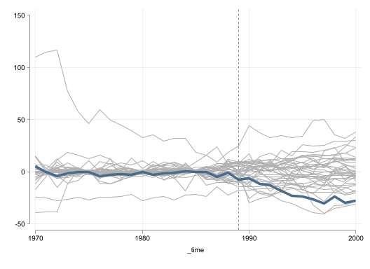
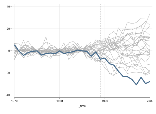
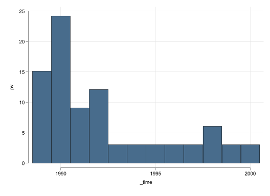
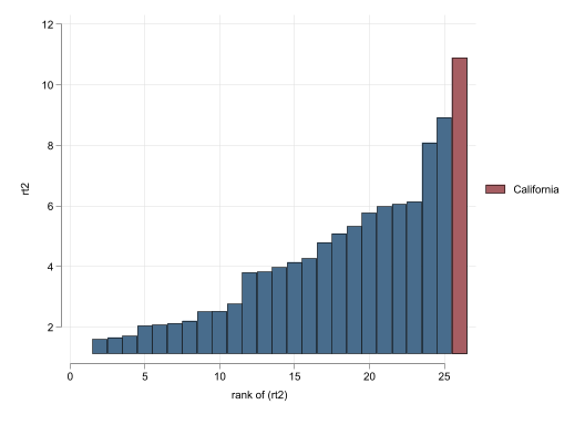
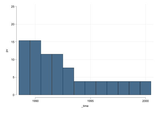
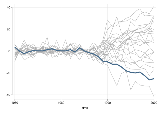
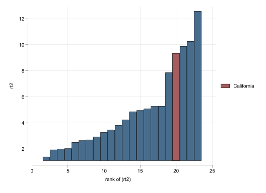
Based on Figure 1, there is an effect of the Policy which reduced sales of cigarates. Figure 1 (c) and Figure 1 (d) suggest the effect is significant across most post-treatment periods.
Log Case
Lets make one change. Instead of using cigarette sale per capita, I will use the log of that variable. The idea is that while raw data may not be comparable, because of different scales across units, data may be more comparable if its comparessed using a logScale.
Interestingly enough Figure 2 shows a very similar effect plot as in Figure 1. The RMSE ratio is even better, but with few post-treatment effects that are not as significant.
Relative Change
The next alternative is to use a relative rescaling. Specifically, I will change the baseline of cigsales across all States, so that Cigarette Sales in 1970 is normalized to be 100. The changes, then could be interpreted in units relative to what happened in 1970.
Based on Figure 3, we still have many states with very bad model fitness. Figure 3 (c) and Figure 3 (d), however, still shows good model performance, with slighly higher significance than when the data was used as is.
Fully Rescale (to California pre-treament)
The last transformation I implement is one where all data is rescaled and shifted so that all countries have the same average and standard deviation in the period before treatment. I believe this could be the best approach, because forces all data to be perfectly comparable in the pre-treatment period, increasing the posibility to find good controls even for the other wise extreme states.
Figure 4: Synthetic Control Results: Rescale to California
What I consider quite interesting is that even the effect plot that uses no restrictions shows very good pre-treatment model fit for all donor units. Although the fitness for California is even better. Once we impose the same restriction to the data, excluding units with a RMSE twice as large as the one in California, we obtain a plot similar to the ones in the previous cases.
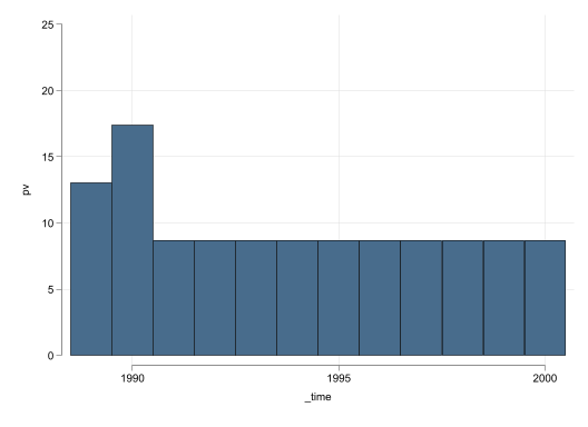
Figure 4 (c) and Figure 4 (d) show that the effect may not be as strong as in the previous example. The RMSE ratio method suggests a p-value of 12.5%, above the standard 5% we like to consider as minimum threshold. The significance across periods is also slighly worse, because there is one state that exhibits a pseudo treatment that is larger than California.
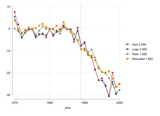
Perhaps what would be the best way to comapre the different cases presented above is to rescale the results as to obtain results that can be compared across specifications. In Figure 5, I puts together this effects, so that they can be compared across each other.
Interestingly enough, Model Specification does very little on the estimated effect, as they all suggest a sharp decline in Cigarette sales of just above 10 fewer packs per capita 3 years after implementation, up to 25/27 fewer packs per capita by 2000.
Asis and Logs specifications show the largest decline in 1997 (30 fewer packs), with rescaled and rate specifications being the most conservative. The table also provides the pre-RMSE for all models. They suggest that using Rates provided the best fit, followed by the ReScaled data, using data as is, and using the log transformation.
Conclusions
This was an interesting excercise driven by asking if it matter how the covariates are measured when applying SC. I was also curious about this approach, as I was trying to understand one of the extensions of the methodology: Synthetid Differences in Differences. This may require some testing, but that can be left for a future exploration.
It may seem, for this simplified example, that it doesnt really matter how covariates are transformed. The estimated effects were effectively the same. This conclusion, however, may not be valid in more complex settings.
Perhaps the only concern at this point is that the “significance” level of the estimates did change considerably with the data rescaling approach. Granted, the change seems large, because the sample is small (25 observations), and a single change in ranking may look like a large change in the p-value of the statistic.
If you are reading this, and have some comments, please let me know.
Source Code
---title: "Synthetic Control: Role of rescaling"description: "I discuss the role of variable transformations on the use of Synthetic control for Causal Analysis"author: "Fernando Rios-Avila"date: "5/9/2023"categories: - Stata - Programming - Causal effectsdraft: false---## IntroductionAs a wise man once said:> **The best way to learn something is to teach it.** Not sure who said that, but I find it to be true, except for instances when the learning process puts you in a position where you have a question, but you do not know how to find an answer. This is one of those ocasions.As some of you may know, the technique known as **Synthetic Control** is a widely recognized methodology used to determine the effects of a treatment on a single treated entity. It accomplishes this by identifying the optimal combination of control variables that form a synthetic control.The purpose of this SControl is to provide an answer to the question of "What would have happened to the treated group **if** no treatment had been administered?" However, when dealing with a single unit of interest, there is a risk of mistaking random fluctuations with the actual treatment effect. To mitigate this risk one may run a set of placebo tests. One of them involves estimating pseudo treatment effects for each individual "control" unit. Ideally, if the controls were adequate, there should be no discernible effect among them. If the impact on the treated group is significant or unusual enough, we could conclude that there is an effect beyond random chance or noise.Because the optimal weights are such you can only construct synthetic controls via interpolation, rather than extrapolation, the estimation of synthetic controls for some of the non-treated units can be difficult. *Unique* units may serve well as controls, but are not suitable as *treated* unit, because no interpolation of data can simulate those units. Because of this, its recommended that one excludes those units when analyzing the significance of the treatment effect.## How does SC works?The basic implementation of SC involves finding a set of optimal weights $w$ such that:$$w^*=\min_w \sum_{h} \left(X_{1,h}-\sum_{j=2}^J w_j X_{j,h}\right)^2$$where $X's$ is a set of pre-treatment characteristics we would like to equalize between the treated unit and the control units. $X$ can contain pretreament outcome characteristics. We also require $\sum w_j =1$ and $w_j\geq 0$. Once the weights have been estimated, we can estimate the treatment effect at any point in time simply as:$$ \tau_t = Y_{1,t}-\sum_{j=2}^J w^*_j \times Y_{j,t}$$## The question without an answerSomething that seems interesting to me is that the construction of treatment effects, or estimation of optimal weights say nothing about how should data be used, nor which variation should we be interested in.Granted, standard approach is to just use data asis, but that seems unsatisfactory. Consider, for example, a case when the interest is on analyzing the effect on GDP of a country level policy in the US. The US being one of the largest economies in the world, it would be difficult, if not impossible to, ex ante, find good controls.But what if we change the measure of interest? and look into GDP percapita, or GDP relative levels, or something else. After the estimation is done, we could certainly reconstruct the original question. Implementing these kind of transformations would help finding better controls, but could have important impacts when estimating the placebo tests assessing the significance of the estimated effect. Here the question:> **To what extend can we transform our explanatory variables when implementing SC**> **Would the transformations need to be the same for all units? or panel units?**Below, I show an example of what could happen when we make these decisions:## Smoking in CaliforniaFor the example I have in mind, I will use the **`Smoking`** dataset that is typically used to teach the methodology. I will also use two community-contributed programs `synth` and `frause`. The second one, just to make it easy uploading the data. I will also use a small programm to prepare the data before creating the figures. This one is rather long, but if you are interested, please take a look.```{stata}*| code-fold: trueset scheme white2capture program drop sc_doerprogram sc_doer** Estimates the Effect for California. tempfile sc3 synth cigsale cigsale(1971) cigsale(1975) cigsale(1980) cigsale(1985), trunit(3) trperiod(1989) keep(`sc3') replace ** And all other states forvalues i =1/39{ if `i'!=3 { local pool foreach j of local stl { if `j'!=3 & `j'!=`i' local pool `pool' `j' } tempfile sc`i' synth cigsale cigsale(1971) cigsale(1975) cigsale(1980) cigsale(1985) , /// trunit(`i') trperiod(1989) keep(`sc`i'') replace counit(`pool') } }** Collects the Saved files to estimate the Treatment effect** and the p-value/ratio statistic forvalues i =1/39{ use `sc`i'' , clear gen tef`i' = _Y_treated - _Y_synthetic egen sef`i'a =mean( (_Y_treated - _Y_synthetic)^2) if _time<=1988 egen sef`i'b =mean( (_Y_treated - _Y_synthetic)^2) if _time>1988 gen sef`i'aa=sqrt(sef`i'a[2]) gen sef`i'bb=sqrt(sef`i'b[_N]) replace sef`i'a=sef`i'aa replace sef`i'b=sef`i'bb drop if _time==. keep tef`i' sef`i'* _time save `sc`i'', replace } clear use `sc1' forvalues i = 2/39 { merge 1:1 _time using `sc`i'', nogen } global toplot global toplot2** Stores which models will be saved for plotting forvalues i = 1/39 { global toplot $toplot (line tef`i' _time, color(gs11) ) if (sef`i'a[1])<(2*sef3a[1]) { global toplot2 $toplot2 (line tef`i' _time, color(gs11) ) } }** Estimates the post/pre RMSE ratio capture matrix drop rt forvalues i = 1/39 { if (sef`i'a[1])<(2*sef3a[1]) { matrix rt=nullmat(rt)\[`i',sef`i'b[1]/sef`i'a[1]] } } svmat rt egen rnk=rank(rt2)** and the ranking /p-value for each period gen rnk2=0 forvalues i = 1/39 { if (sef`i'a[1])<(2*sef3a[1]) { local t = `t'+1 replace rnk2=rnk2+(tef`i'<=tef3) } } gen pv=rnk2*100/`t'end```### ASIS caseThe first case will be the "vanilla" one. I will only use 4 pretreatment outcomes for the weight construction: 1971, 1975, 1980 and 1985. The outcome of interest is cigarette sale per capita (in packs). Thus, to some extend, data has already been standardized to be measured in comparable units.The basic code will look like this:```statasynth cigsale cigsale(1971) cigsale(1975) cigsale(1980) cigsale(1985), trunit(3) trperiod(1989) ``````{stata}qui:frause smoking2, clearqui:xtset state yearqui:sort state yearqui:sc_doer```which will produce the following:```{stata}*| label: fig-sc1*| fig-cap: "Synthetic Control Results: ASIS"*| fig-subcap:*| - Unrestricted effect*| - Restricted effect*| - RMSE Ratio*| - P-value*| layout-ncol: 2*| layout-nrow: 2*| column: pagetwo $toplot (line tef3 _time, lw(1) color(navy*.8)), xline(1989) legend(off) name(m1, replace)two $toplot2 (line tef3 _time, lw(1) color(navy*.8)), xline(1989) legend(off) name(m2, replace)two bar rt2 rnk || bar rt2 rnk if rt1==3 , legend(order( 2 "California")) name(m3, replace)two bar pv _time if _time>1988 & pv<40, legend(off) name(m4, replace) ylabel(0(5)25)```Based on @fig-sc1, there is an effect of the Policy which reduced sales of cigarates. @fig-sc1-3 and @fig-sc1-4 suggest the effect is significant across most post-treatment periods.### Log CaseLets make one change. Instead of using cigarette sale per capita, I will use the log of that variable. The idea is that while raw data may not be comparable, because of different scales across units, data may be more comparable if its comparessed using a logScale.```{stata}*| code-fold: true*| echo: falsequi:frause smoking2, clearqui:xtset state yearqui:sort state yearqui:replace cigsale=log(cigsale)qui:sc_doer``````{stata}*| label: fig-sc2*| fig-cap: "Synthetic Control Results: Logs"*| fig-subcap:*| - Unrestricted effect*| - Restricted effect*| - RMSE Ratio*| - P-value*| layout-ncol: 2*| layout-nrow: 2*| column: pagetwo $toplot (line tef3 _time, lw(1) color(navy*.8)), xline(1989) legend(off) name(m1, replace)two $toplot2 (line tef3 _time, lw(1) color(navy*.8)), xline(1989) legend(off) name(m2, replace)two bar rt2 rnk || bar rt2 rnk if rt1==3 , legend(order( 2 "California")) name(m3, replace)two bar pv _time if _time>1988 & pv<40, legend(off) name(m4, replace) ylabel(0(5)25)```Interestingly enough @fig-sc2 shows a very similar effect plot as in @fig-sc1. The RMSE ratio is even better, but with few post-treatment effects that are not as significant.### Relative ChangeThe next alternative is to use a relative rescaling. Specifically, I will change the baseline of cigsales across all States, so that Cigarette Sales in 1970 is normalized to be 100. The changes, then could be interpreted in units relative to what happened in 1970.```{stata}*| code-fold: true*| echo: falsequi:frause smoking2, clearqui:xtset state yearqui:sort state yearqui:by state:replace cigsale=cigsale/cigsale[1]*100qui:sc_doer``````{stata}*| label: fig-sc3*| fig-cap: "Synthetic Control Results: Logs"*| fig-subcap:*| - Unrestricted effect*| - Restricted effect*| - RMSE Ratio*| - P-value*| layout-ncol: 2*| layout-nrow: 2*| column: pagetwo $toplot (line tef3 _time, lw(1) color(navy*.8)), xline(1989) legend(off) name(m1, replace)two $toplot2 (line tef3 _time, lw(1) color(navy*.8)), xline(1989) legend(off) name(m2, replace)two bar rt2 rnk || bar rt2 rnk if rt1==3 , legend(order( 2 "California")) name(m3, replace)two bar pv _time if _time>1988 & pv<40, legend(off) name(m4, replace) ylabel(0(5)25)```Based on @fig-sc3, we still have many states with very bad model fitness. @fig-sc3-3 and @fig-sc3-4, however, still shows good model performance, with slighly higher significance than when the data was used as is.### Fully Rescale (to California pre-treament)The last transformation I implement is one where all data is rescaled and shifted so that all countries have the same average and standard deviation in the period before treatment. I believe this could be the best approach, because forces all data to be perfectly comparable in the pre-treatment period, increasing the posibility to find good controls even for the other wise extreme states.```{stata}*| code-fold: true*| echo: falsequi:frause smoking, clearqui:xtset state yearqui:sort state yearqui{ sum cigsale if state==3 & year<=1988 local cmean=r(mean) local smean=r(sd) forvalues i = 1/39 { sum cigsale if state==`i' & year<=1988 replace cigsale = `cmean' + `smean' * (cigsale - r(mean))/r(sd) if state==`i' }}qui:sc_doer``````{stata}*| label: fig-sc4*| fig-cap: "Synthetic Control Results: Rescale to California"*| fig-subcap:*| - Unrestricted effect*| - Restricted effect*| - RMSE Ratio*| - P-value*| layout-ncol: 2*| layout-nrow: 2*| column: pagetwo $toplot (line tef3 _time, lw(1) color(navy*.8)), xline(1989) legend(off) name(m1, replace)two $toplot2 (line tef3 _time, lw(1) color(navy*.8)), xline(1989) legend(off) name(m2, replace)two bar rt2 rnk || bar rt2 rnk if rt1==3 , legend(order( 2 "California")) name(m3, replace)two bar pv _time if _time>1988 & pv<40, legend(off) name(m4, replace) ylabel(0(5)25)frame put *, into(m4)```What I consider quite interesting is that even the effect plot that uses no restrictions shows very good pre-treatment model fit for all donor units. Although the fitness for California is even better. Once we impose the same restriction to the data, excluding units with a RMSE twice as large as the one in California, we obtain a plot similar to the ones in the previous cases.@fig-sc4-3 and @fig-sc4-4 show that the effect may not be as strong as in the previous example. The RMSE ratio method suggests a p-value of 12.5%, above the standard 5% we like to consider as minimum threshold. The significance across periods is also slighly worse, because there is one state that exhibits a pseudo treatment that is larger than California. ## Comparing Magnitude effects```{stata}*| output: false*| code-fold: true*| echo: truequi:frause smoking2, cleartempfile sc1x sc2x sc3x sc4xxtset state yearqui: { gen or_cigsale=cigsale synth cigsale cigsale(1971) cigsale(1975) cigsale(1980) cigsale(1985), trunit(3) trperiod(1989) keep(`sc1x') replace replace cigsale=log(or_cigsale) synth cigsale cigsale(1971) cigsale(1975) cigsale(1980) cigsale(1985), trunit(3) trperiod(1989) keep(`sc2x') replace sort state year by state:replace cigsale=or_cigsale/or_cigsale[1]*100 synth cigsale cigsale(1971) cigsale(1975) cigsale(1980) cigsale(1985), trunit(3) trperiod(1989) keep(`sc3x') replace sum or_cigsale if state==3 & year<=1988 local cmean=r(mean) local smean=r(sd) forvalues i = 1/39 { sum or_cigsale if state==`i' & year<=1988 replace cigsale = `cmean' + `smean' * (or_cigsale - r(mean))/r(sd) if state==`i' } synth cigsale cigsale(1971) cigsale(1975) cigsale(1980) cigsale(1985), trunit(3) trperiod(1989) keep(`sc4x') replace }clearuse `sc1x'rename _Y_synthetic y1_synthdrop if _time==.save `sc1x', replaceuse `sc2x'rename _Y_synthetic y2_synthreplace y2_synth = exp(y2_synth )drop if _time==.save `sc2x', replaceuse `sc3x'ren _Y_synthetic y3_synthdrop if _time==.save `sc3x', replaceuse `sc4x'ren _Y_synthetic y4_synthdrop if _time==.save `sc4x', replaceuse `sc1x', clearmerge 1:1 _time using `sc2x', nogenmerge 1:1 _time using `sc3x', nogenmerge 1:1 _time using `sc4x', nogenreplace y3_synth=y3_synth* _Y_treated[1]/100gen eff1= _Y_treated-y1_synthgen eff2= _Y_treated-y2_synthgen eff3= _Y_treated-y3_synthgen eff4= _Y_treated-y4_synth```Perhaps what would be the best way to comapre the different cases presented above is to rescale the results as to obtain results that can be compared across specifications. In @fig-sc5, I puts together this effects, so that they can be compared across each other. ```{stata}*| label: fig-sc5*| fig-cap: "Synthetic Control Effects"scatter eff* _time, connect(l l l l) msymbol(O D T S) xline(1989) ///legend(order(1 "Asis 2.550" 2 "Logs 2.859" 3 "Rate 1.928" 4 "Rescaled 1.955"))```Interestingly enough, Model Specification does very little on the estimated effect, as they all suggest a sharp decline in Cigarette sales of just above 10 fewer packs per capita 3 years after implementation, up to 25/27 fewer packs per capita by 2000. Asis and Logs specifications show the largest decline in 1997 (30 fewer packs), with rescaled and rate specifications being the most conservative. The table also provides the pre-RMSE for all models. They suggest that using Rates provided the best fit, followed by the ReScaled data, using data as is, and using the log transformation.## ConclusionsThis was an interesting excercise driven by asking if it matter how the covariates are measured when applying SC. I was also curious about this approach, as I was trying to understand one of the extensions of the methodology: Synthetid Differences in Differences. This may require some testing, but that can be left for a future exploration.It may seem, for this simplified example, that it doesnt really matter how covariates are transformed. The estimated effects were effectively the same. This conclusion, however, may not be valid in more complex settings. Perhaps the only concern at this point is that the "significance" level of the estimates did change considerably with the data rescaling approach. Granted, the change seems large, because the sample is small (25 observations), and a single change in ranking may look like a large change in the p-value of the statistic.If you are reading this, and have some comments, please let me know.