Nonlinear DID

Lessons from Staggered Linear Differences in Differences

Author

Affiliation

Fernando Rios-Avila

Levy Economics Institute

Introduction

Differences in Differences (DiD) design is one of the most popular methods in applied microeconomics, because it requires relatively few assumptions to identify treatment effects.
- No anticipation,
- Parallel trends,
- No spillovers
The canonical DiD, a 2x2 design, simply compares means (or conditional means) of the outcome variable (before after x treated non-treated) to identify treatment effects.
- Thus it can be used even if outcome is a limited dependent variable (binary, count, etc) (parallel to the linear regression case)

Because the Canonical design is rather limited, many extensions have been proposed to handle more complex scenarios: Staggered Treatment with GxT DID.
- Early Extensions (infamous TWFE) have been shown to be problematic. (negative weights and bad controls)
- but more recent approaches (See Roth et al. (2023)) have shown how can one better use these designs to identify treatment effects, avoiding the simple-TWFE problems.
Linear models, however, have limitations:
- Linear models do a poor job interpolating and predicting LDV outcomes
- Parallel trends assumptions may only be credible under specific functional forms

Disclaimer:

who am I not?

Not Andrew Goodman-Bacon

Among others, Andrew showed the problems of using TWFE in the presence of staggered adoption of the treatment.
Because of treatment timing, later treated units are compared to bad controls (early treated ones), in potential violation of the parallel trends assumption.
This also relates to negative weights.
See Goodman-Bacon (2021)

Not Pedro Sant’Anna

Pedro and Brantly proposed deconstructing the GxT problem. Consider only good 2x2 DD designs to identify Treatment effects in DID.
Agregate them as needed to obtain the desired treatment effect (weighted Average). (dynamic, average, across time, across groups, etc)
Along with Jonathan Roth, discuss the problem of PTA and functional forms. Not all may be valid.
see Callaway and Sant’Anna (2021) and Roth and Sant’Anna (2023)

Not Jeffrey Wooldridge

Jeff Wooldridge brought back life to the TWFE.
The problem was not the TWFE part of the analysis, but the model specification.
- (\(post \times treated\) instead of \(G \times T\))
This insights, can be extended to nonlinear cases.
See Wooldridge (2021) and Wooldridge (2023)

Fernando Rios-Avila

I have followed some of the developments in DID with staggered adoption of the treatment.
- Implemented few things (drdid/csdid/csdid2/jwdid)
- Understood few others (comparison groups, efficiency, negative weights, nonlinear models)
And today, I will be providing some of my insights regarding the empirical analysis of nonlinear DID.
- I will rely heavily on Wooldridge (2023),

Basics: 2x2 DiD

In the 2x2 DID design, we have 2 groups:
- Control (\(D=0\)) and treated (\(D=1\)),
Which are observed for two periods of time:
- Before (\(T=0\)) and after (\(T=1\)) the treatment.
For all groups and periods of time, we observe the realized outcome \(Y_{i,t}\), but cannot observe all potential outcomes \(Y_{i,t}(D)\).
Realized outcomes are determined by the following equation:

\[Y_{i,t}=D_i Y_{i,t}(1) + (1-D_i) Y_{i,t}(0) \]

If treatment occured at some point between T0 and T1, and we could observe all potential outcomes, the estimate of interested, Average Treatment effect, could be estimated as follows:

\[ATT = E(Y_{i,1}(1) - Y_{i,1}(0)|D_i=1) \]

For the treated, we observe \(Y_{i,1}(1)\), but cannot observe \(Y_{i,t}(0)\) (counterfactual), thus, to identify Treatment Effects, we need to impose some assumptions.

PTA:

\[\begin{aligned} E(Y_{i,1}(0) - Y_{i,0}(0)|D_i=1) &= E(Y_{i,1} - Y_{i,0}|D_i=0) \\ E(Y_{i,1}(0)|D_i=1) &= E(Y_{i,0}(0)|D_i=1) + E(Y_{i,1} - Y_{i,0}|D_i=0) \end{aligned} \]

No Anticipation: \[Y_{i,0}(1) = Y_{i,0}(0)=Y_{i,0}\]

Thus, ATT can be estimated as follows:

\[\begin{aligned} ATT &= E(Y_{i,1}(1)|D_i=1)-E(Y_{i,1}(0)|D_i=1) \\ &= E(Y_{i,1}|D_i=1)- \Big(E(Y_{i,0}|D_i=1) + E(Y_{i,1} - Y_{i,0}|D_i=0) \Big) \\ &= E(Y_{i,1}-Y_{i,0}|D_i=1)- E(Y_{i,1} - Y_{i,0}|D_i=0) \end{aligned} \]

And the Same could be done via Regressions:

\[y_{i,t} = \beta_0 + \beta_1 T + \beta_2 D_i + \theta (D_i \times T) + \epsilon_{i,t} \]

ATT identification relies on the Parallel trend assumption.

How to test for PTA?

PTA is a non-testable assumption, because we do not observe all potential outcomes.
However, if we “move”, from the 2x2 design, it may be possible to test if PTA hold Before treatment.
Consider a case of T periods of time, and that treatment happen at period G.
Say we estimate the ATT comparing periods T and T-1, for any T<G.

\[ATT(T) = E(Y_{i,T} - Y_{i,T-1}|D_i=1) - E(Y_{i,T} - Y_{i,T-1}|D_i=0) \]

If there is no anticipation, and Parallel trends hold, then \(ATT(T)=0 \text{ if } T<G\)
- This is what Callaway and Sant’Anna (2021) uses for PTA testing

How to test for PTA?

Alternatively, one could simply estimate all ATT’s using period G-1 as baseline period (long2 differences):

\[ATT^2(T) = E(Y_{i,T} - Y_{i,G-1}|D_i=1) - E(Y_{i,T} - Y_{i,G-1}|D_i=0) \]

And use all post-treatment periods to estimate the ATT (\(T\geq G\))
and use all pre-treatment periods to test for PTA (\(T<G\))

As suggested by Wooldridge (2023), one of the reasons PTA may not hold is because we may be analyzing the wrong model.
- consider two groups of workers, high and low earners, that experience the same wage growth. (parallel trends in relative terms)
- If we observe wages at levels, parallel trends would be violated
- And Post treatment estimates will be missleading

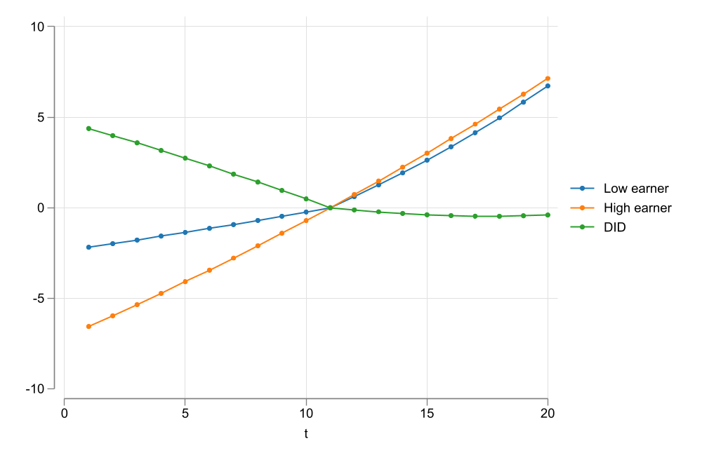
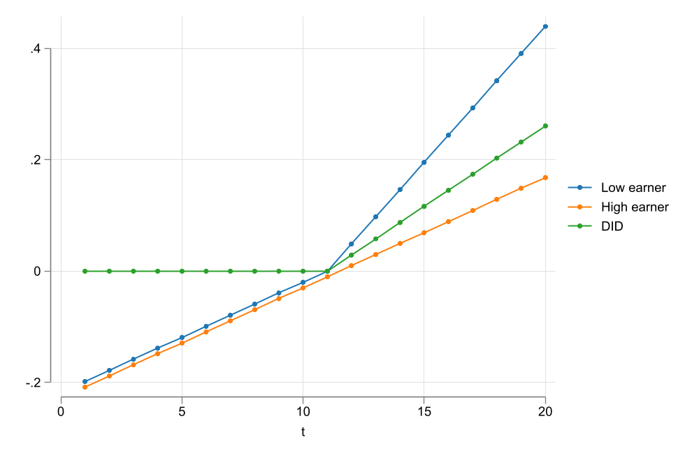
PTA may hold for \(G(\bar Y)\)

A similar story could be told about other types of transformations.

In general, it is possible that PTA hold for some other monotonic transformation of the outcome variable.

\[G^{-1}\Big( E_1 [Y_{i,1}(0)] \Big) -G^{-1}\Big(E_1[ Y_{i,0}(0) ] \Big) = G^{-1}\Big(E_0[Y_{i,1}]\Big) - G^{-1}\Big(E_0[Y_{i,0}]\Big) \]

This is very similar to the PTA assumption explored in Roth and Sant’Anna (2023).

\[E_1\Big[g(Y_{i,1}(0))\Big] - E_1\Big[g(Y_{i,0}(0))\Big] = E_0\Big[g(Y_{i,1})\Big] - E_0\Big[g(Y_{i,0})\Big] \]

Wooldridge idea: It may be possible to identify ATTs using correct functional forms, through the latent index.

How do things Change?

Using this insight, we can go back to the 2x2 design, and see how things change.

Before:

\[E(y_{i,t}|D,T)=\beta_0 + \beta_1 T + \beta_2 D_i + \theta (D_i \times T) \]

After:

\[E(y_{i,t}|D,T)=G\Big(\beta_0 + \beta_1 T + \beta_2 D_i + \theta (D_i \times T)\Big) \]

For the practitioner, the extended Nonlinear DID simply requires choosing a functional form that better fits the data.
- Poisson, logit, ~~fractional regression~~, multinomial model, Linear model, etc

Extension I: Adding Covariates

Many papers in the literature consider the use of covariates in the estimation of the ATT.
The lessons from Sant’Anna and Zhao (2020):
- The choosen covariates should be time fixed, to avoid contamination of the treatment effect.
- Using covariates allows relaxing the parallel trends assumption: PTA hold for specific groups of individuals. (if not for the whole population due to compositional changes)
In the 2x2 DID-Regression, covariates can be added with interactions:

\[\begin{aligned} y_{i,t} &= \beta_0 + \beta_1 D + \beta_2 T + \theta (D \times T) \\ &+ X\gamma + D \times X\gamma_d + T \times X\gamma_T + D \times T (X-\bar X )\lambda + \epsilon_{i,t} \end{aligned} \]

The same could be done in the nonlinear case

Extension II: GxT DiD

The 2x2 design is rather limited, because often people have access to multiple periods of time, with differential treatment timing. (staggered adoption of the treatment)
- I call this the GxT design (G groups, T periods of time)
The majority of the papers that analyze this case impose an additional assumption:
- Treatment is not Reversable: Once treated always treated

NOTE: Because of the interactions required, adding covariates would rapidily “consume” degrees of freedom. (may be a problem with nonlinear models).

How to see this? --> tab tvar gvar

The Problem

Early extensions of the 2x2 design to the GxT design, relied on the TWFE estimator. \[y_{i,t} = \delta_i + \delta_t + \theta^{fe} D_{i,t} + e_{i,t}\]

where \(D_{i,t}=1\) only after treatment is in place, and zero otherwise.

This model has been shown to be problematic, because of How OLS estimates the \(\theta^{fe}\) parameter.
- \(\theta^{fe}\) is a weighted average of all possible 2x2 DID designs. Goodman-Bacon (2021)
- Some designs use early treated units as controls for late treated units, which might be a violation of the parallel trends assumption.
  - (treated units effectively receiving negative weights) Goodman-Bacon (2021), Chaisemartin and D’Haultfœuille (2020) and Borusyak, Jaravel, and Spiess (2023).

Avoiding the Problem

Callaway and Sant’Anna (2021) proposes a simple solution: Deconstruct the problem into smaller pieces (2x2 DIDs), and aggregate them as needed.
Wooldridge (2021), however, proposes a different solution: Use the correct functional form to estimate the ATTs.

\[\text{Instead of: }Y_{i,t} = \delta_i + \gamma_t + \theta^{fe} PT_{i,t} + \epsilon_{i,t}\]

\[\text{Use: }Y_{i,t} = \delta_i + \gamma_t + \sum_{g \in \mathbb{G}} \sum_{t=g}^T \theta_{g,t} \mathbb{1}(G=g,T=t) + \epsilon_{i,t}\]

Their Message: Embrace heterogeneity across time and cohorts.

An added Insight

The approach proposed by Wooldridge (2021), is more efficient than Callaway and Sant’Anna (2021), because it uses all pre-treatment data to estimate the ATTs. (Callaway and Sant’Anna (2021) uses only one pre-treatment period)
However, doing this doesn’t allow you to test for PTA directly, unless we use an alternative approach:

\[Y_{i,t} = \delta_i + \gamma_t + \sum_{g \in \mathbb{G}} \sum_{t=t_0}^{g-2} \theta_{g,t}^{pre} \mathbb{1}(G=g,T=t) + \sum_{g \in \mathbb{G}} \sum_{t=g}^T \theta_{g,t}^{post} \mathbb{1}(G=g,T=t) + \epsilon_{i,t}\]

This specification is equivalent to Callaway and Sant’Anna (2021) and to Sun and Abraham (2021).
- Its explicily a regression (Wooldridge)
- and uses actual, instead of relative, time.

Implementing NL-DID the `JW` way

One of the advantages of the approaches proposed by Wooldridge (2021) and Wooldridge (2023), is that they can be directly estimated using regressions.
The hard part is to construct all the interactions required for the model to work.
And a second challenge is to aggregate the results.

jwdid

jwdid is a simple command that helps with the construction of all required interactions that could be used to implement Wooldridge approach.
It is flexible enough, in that it allows you to choose different estimators that would better fit your data.
it comes with its own post estimation commands that can help you aggregate the results into simple ATT, dynamics effects, across periods, across years, etc.
Lets take it for a spin

Command Syntax

jwdid - Command Name. In charge of getting all interactions -right-
- depvar [indepvar] - Declare the dependent variables. Independent variables are optional. They should be time fixed.
- [if] [in] [weight], Declares sample and weights. Only PW is allowed.

Command Main Options

jwdid: main options
- ivar(varname): Panel indicator. If not declared, command assumes one is using repeated cross sections.
- cluster(varname): Cluster variable. To request a clustered standard error other than at ivar level. Recommended with RC.
- tvar(varname) or time(varname): Required, Time variable. There are two ways to call it for compatability with csdid.
- gvar(varname): Group variable. Indicates the timing of when a unit has ben treated.
- trtvar(varname): If using Panel data, one could instead provide the post-treatment dummy.
  - If data is repeated crossection, one requires using trgvar(varname) (Pseudo panel indicator).

Extra Options

group: Requests using group fixed effects, instead of individual fixed effects (default)
never: Request to use alternative specification that allows to test for PTA. (default is to use the standard specification)
Linear and Nonlinear models:
- method(command, options): Request to use a specific method to model the data. Default is using linear regression via reghdfe.
- the option part allows you do include specific options for the method. (e.g. method(glm, link() family()))

Example 1: Min Wages on Employment CS data

clear all
qui:ssc install frause
qui:frause mpdta, clear
frause mpdta, clear
jwdid lemp, ivar(county) tvar(year) gvar(first)

(Written by R.              )
WARNING: Singleton observations not dropped; statistical significance is biased
>  (link)
(MWFE estimator converged in 2 iterations)

HDFE Linear regression                            Number of obs   =      2,500
Absorbing 2 HDFE groups                           F(   7,    499) =       3.82
Statistics robust to heteroskedasticity           Prob > F        =     0.0005
                                                  R-squared       =     0.9933
                                                  Adj R-squared   =     0.9915
                                                  Within R-sq.    =     0.0101
Number of clusters (countyreal) =        500      Root MSE        =     0.1389

                           (Std. err. adjusted for 500 clusters in countyreal)
------------------------------------------------------------------------------
             |               Robust
        lemp | Coefficient  std. err.      t    P>|t|     [95% conf. interval]
-------------+----------------------------------------------------------------
 first_treat#|
        year#|
    c.__tr__ |
  2004 2004  |  -.0193724   .0223818    -0.87   0.387    -.0633465    .0246018
  2004 2005  |  -.0783191   .0304878    -2.57   0.010    -.1382195   -.0184187
  2004 2006  |  -.1360781   .0354555    -3.84   0.000    -.2057386   -.0664177
  2004 2007  |  -.1047075   .0338743    -3.09   0.002    -.1712613   -.0381536
  2006 2006  |   .0025139   .0199328     0.13   0.900    -.0366487    .0416765
  2006 2007  |  -.0391927   .0240087    -1.63   0.103    -.0863634     .007978
  2007 2007  |   -.043106   .0184311    -2.34   0.020    -.0793182   -.0068938
             |
       _cons |    5.77807    .001544  3742.17   0.000     5.775036    5.781103
------------------------------------------------------------------------------

Absorbed degrees of freedom:
-----------------------------------------------------+
 Absorbed FE | Categories  - Redundant  = Num. Coefs |
-------------+---------------------------------------|
  countyreal |       500         500           0    *|
        year |         5           0           5     |
-----------------------------------------------------+
* = FE nested within cluster; treated as redundant for DoF computation

gen emp = exp(lemp)
jwdid emp, ivar(county) tvar(year) gvar(first) method(poisson)


Iteration 0:   log pseudolikelihood = -2980537.4  
Iteration 1:   log pseudolikelihood = -2980526.5  
Iteration 2:   log pseudolikelihood = -2980526.5  

Poisson regression                                      Number of obs =  2,500
                                                        Wald chi2(14) = 225.38
Log pseudolikelihood = -2980526.5                       Prob > chi2   = 0.0000

                           (Std. err. adjusted for 500 clusters in countyreal)
------------------------------------------------------------------------------
             |               Robust
         emp | Coefficient  std. err.      z    P>|z|     [95% conf. interval]
-------------+----------------------------------------------------------------
 first_treat#|
        year#|
    c.__tr__ |
  2004 2004  |  -.0080499   .0100858    -0.80   0.425    -.0278177    .0117178
  2004 2005  |  -.0252131   .0176754    -1.43   0.154    -.0598562    .0094299
  2004 2006  |   -.051965   .0197745    -2.63   0.009    -.0907222   -.0132077
  2004 2007  |  -.0672208   .0192207    -3.50   0.000    -.1048926    -.029549
  2006 2006  |    .055212   .0330023     1.67   0.094    -.0094714    .1198954
  2006 2007  |   .0109993     .04294     0.26   0.798    -.0731617    .0951602
  2007 2007  |   -.060675   .0149793    -4.05   0.000    -.0900339   -.0313161
             |
 first_treat |
       2004  |   .4789133   .4347691     1.10   0.271    -.3732184    1.331045
       2006  |   .6010118   .3248861     1.85   0.064    -.0357532    1.237777
       2007  |   .1269293   .2472938     0.51   0.608    -.3577576    .6116163
             |
        year |
       2004  |  -.0459369   .0064592    -7.11   0.000    -.0585966   -.0332771
       2005  |  -.0301284   .0094457    -3.19   0.001    -.0486416   -.0116152
       2006  |  -.0030985   .0122001    -0.25   0.800    -.0270104    .0208133
       2007  |   .0350031   .0118264     2.96   0.003     .0118238    .0581824
             |
       _cons |    6.84775   .1555219    44.03   0.000     6.542932    7.152567
------------------------------------------------------------------------------

jwdid emp, ivar(county) tvar(year) gvar(first) method(poisson) never


Iteration 0:   log pseudolikelihood = -2980450.1  
Iteration 1:   log pseudolikelihood = -2980438.8  
Iteration 2:   log pseudolikelihood = -2980438.8  

Poisson regression                                      Number of obs =  2,500
                                                        Wald chi2(19) = 262.50
Log pseudolikelihood = -2980438.8                       Prob > chi2   = 0.0000

                           (Std. err. adjusted for 500 clusters in countyreal)
------------------------------------------------------------------------------
             |               Robust
         emp | Coefficient  std. err.      z    P>|z|     [95% conf. interval]
-------------+----------------------------------------------------------------
 first_treat#|
        year#|
    c.__tr__ |
  2004 2004  |  -.0063802   .0111509    -0.57   0.567    -.0282356    .0154752
  2004 2005  |   -.027483   .0190781    -1.44   0.150    -.0648753    .0099094
  2004 2006  |  -.0641446   .0224733    -2.85   0.004    -.1081913   -.0200978
  2004 2007  |  -.0704859   .0204208    -3.45   0.001    -.1105099   -.0304619
  2006 2003  |  -.0081647   .0366458    -0.22   0.824     -.079989    .0636597
  2006 2004  |  -.0289763   .0258763    -1.12   0.263    -.0796929    .0217403
  2006 2006  |   .0310817   .0186723     1.66   0.096    -.0055153    .0676788
  2006 2007  |  -.0042165   .0335939    -0.13   0.900    -.0700593    .0616263
  2007 2003  |   .0358582   .0236868     1.51   0.130    -.0105671    .0822835
  2007 2004  |   .0517571   .0164417     3.15   0.002      .019532    .0839822
  2007 2005  |   .0237174   .0112134     2.12   0.034     .0017395    .0456952
  2007 2007  |  -.0329817    .009941    -3.32   0.001    -.0524657   -.0134976
             |
 first_treat |
       2004  |   .4821784   .4354246     1.11   0.268    -.3712381    1.335595
       2006  |   .6162276   .3252255     1.89   0.058    -.0212028    1.253658
       2007  |    .099236    .244468     0.41   0.685    -.3799124    .5783844
             |
        year |
       2004  |  -.0476066   .0080213    -5.94   0.000     -.063328   -.0318852
       2005  |  -.0278586   .0118649    -2.35   0.019    -.0511134   -.0046038
       2006  |    .009081    .016213     0.56   0.575    -.0226959     .040858
       2007  |   .0382682   .0136908     2.80   0.005     .0114347    .0651017
             |
       _cons |   6.844485   .1573451    43.50   0.000     6.536094    7.152875
------------------------------------------------------------------------------

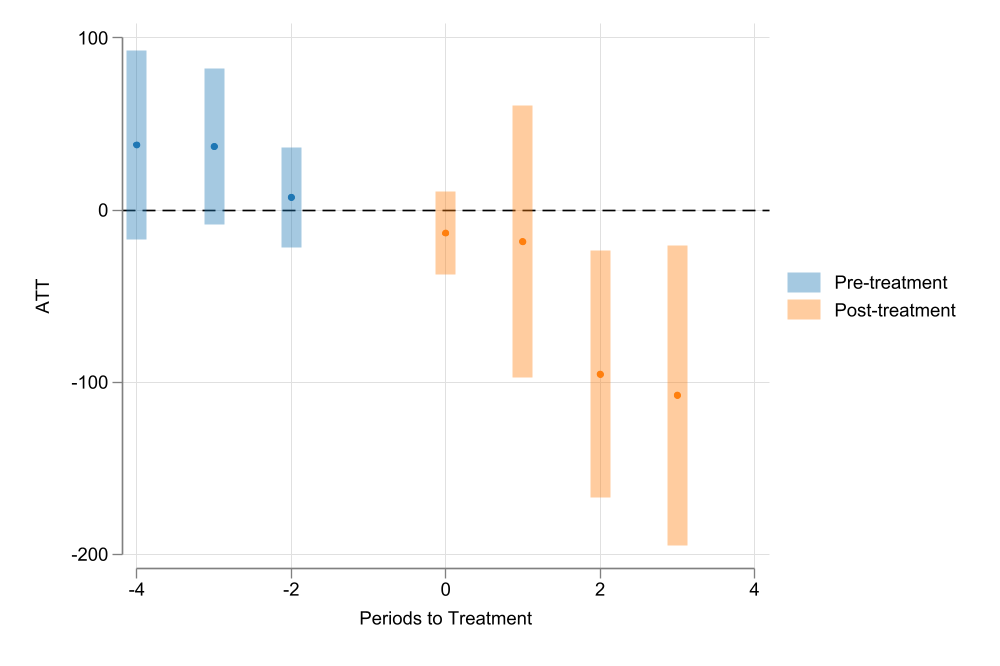
Example 1: Aggregations

estat event

------------------------------------------------------------------------------
             |            Delta-method
             | Coefficient  std. err.      z    P>|z|     [95% conf. interval]
-------------+----------------------------------------------------------------
   __event__ |
         -4  |   37.84578   27.92442     1.36   0.175    -16.88508    92.57665
         -3  |   36.91665   23.13761     1.60   0.111     -8.43224    82.26554
         -2  |   7.462364   14.88422     0.50   0.616    -21.71018    36.63491
         -1  |          0  (omitted)
          0  |  -13.33389   12.32746    -1.08   0.279    -37.49527    10.82749
          1  |  -18.42686   40.35552    -0.46   0.648    -97.52222     60.6685
          2  |   -95.3188   36.54186    -2.61   0.009    -166.9395   -23.69806
          3  |  -107.5067   44.45653    -2.42   0.016    -194.6399   -20.37347
------------------------------------------------------------------------------

estat group

------------------------------------------------------------------------------
             |            Delta-method
             | Coefficient  std. err.      z    P>|z|     [95% conf. interval]
-------------+----------------------------------------------------------------
   __group__ |
       2004  |  -63.03151   28.14208    -2.24   0.025     -118.189   -7.874052
       2006  |   23.89072   46.37715     0.52   0.606    -67.00682    114.7883
       2007  |  -34.94374   13.54265    -2.58   0.010    -61.48686   -8.400625
------------------------------------------------------------------------------

estat calendar

------------------------------------------------------------------------------
             |            Delta-method
             | Coefficient  std. err.      z    P>|z|     [95% conf. interval]
-------------+----------------------------------------------------------------
__calendar__ |
       2004  |  -9.219455   15.81277    -0.58   0.560    -40.21192    21.77301
       2005  |  -40.08113   29.74368    -1.35   0.178    -98.37767    18.21541
       2006  |   5.147843   33.13277     0.16   0.877     -59.7912    70.08689
       2007  |  -36.81546   16.84608    -2.19   0.029    -69.83316   -3.797752
------------------------------------------------------------------------------

qui:estat event, plot
graph export event.png, replace width(1000)

Example 2: Wooldridge Simulation data

clear all
use did_common_6_binary, clear
qui {
reg y i.w#c.d#c.f04 i.w#c.d#c.f05 i.w#c.d#c.f06 ///
    i.w#c.d#c.f04#c.x i.w#c.d#c.f05#c.x i.w#c.d#c.f06#c.x ///
    f02 f03 f04 f05 f06 ///
    c.f02#c.x c.f03#c.x c.f04#c.x c.f05#c.x c.f06#c.x /// 
    d x c.d#c.x, noomitted vce(cluster id)
  est sto m1
}  
qui:margins, dydx(w) at(f02 = 0 f03 = 0 f04 = 1 f05 = 0 f06 = 0) ///
    subpop(if d == 1) noestimcheck vce(uncond)  post
ereturn display  
est restore m1
qui:margins, dydx(w) at(f02 = 0 f03 = 0 f04 = 0 f05 = 1 f06 = 0) ///
    subpop(if d == 1) noestimcheck vce(uncond) post
ereturn display  
est restore m1
qui:margins, dydx(w) at(f02 = 0 f03 = 0 f04 = 0 f05 = 0 f06 = 1) ///
    subpop(if d == 1) noestimcheck vce(uncond) post
ereturn display

                                 (Std. err. adjusted for 1,000 clusters in id)
------------------------------------------------------------------------------
             |            Unconditional
             | Coefficient  std. err.      t    P>|t|     [95% conf. interval]
-------------+----------------------------------------------------------------
         1.w |   .0462206   .0367939     1.26   0.209    -.0259816    .1184228
------------------------------------------------------------------------------
(results m1 are active now)
                                 (Std. err. adjusted for 1,000 clusters in id)
------------------------------------------------------------------------------
             |            Unconditional
             | Coefficient  std. err.      t    P>|t|     [95% conf. interval]
-------------+----------------------------------------------------------------
         1.w |   .0755069   .0376124     2.01   0.045     .0016985    .1493153
------------------------------------------------------------------------------
(results m1 are active now)
                                 (Std. err. adjusted for 1,000 clusters in id)
------------------------------------------------------------------------------
             |            Unconditional
             | Coefficient  std. err.      t    P>|t|     [95% conf. interval]
-------------+----------------------------------------------------------------
         1.w |   .0445457   .0379857     1.17   0.241    -.0299952    .1190866
------------------------------------------------------------------------------

Using jwdid:

clear all
use did_common_6_binary, clear
qui: jwdid y x, ivar(id) tvar(year) trtvar(w) method(regress)
estat event, vce(unconditional)

                                 (Std. err. adjusted for 1,000 clusters in id)
------------------------------------------------------------------------------
             |            Unconditional
             | Coefficient  std. err.      t    P>|t|     [95% conf. interval]
-------------+----------------------------------------------------------------
   __event__ |
          0  |   .0462206   .0367939     1.26   0.209    -.0259816    .1184228
          1  |   .0755069   .0376124     2.01   0.045     .0016985    .1493153
          2  |   .0445457   .0379857     1.17   0.241    -.0299952    .1190866
------------------------------------------------------------------------------

Using Logit

clear all
use did_common_6_binary, clear
qui {
logit y i.w#c.d#c.f04 i.w#c.d#c.f05 i.w#c.d#c.f06 ///
    i.w#c.d#c.f04#c.x i.w#c.d#c.f05#c.x i.w#c.d#c.f06#c.x ///
    f02 f03 f04 f05 f06 c.f02#c.x c.f03#c.x c.f04#c.x c.f05#c.x c.f06#c.x ///
    d x c.d#c.x, noomitted vce(cluster id)
  est store m1
}  

qui:margins, dydx(w) at(f02 = 0 f03 = 0 f04 = 1 f05 = 0 f06 = 0) ///
    subpop(if d == 1) noestimcheck vce(uncond)  post
ereturn display  
est restore m1
qui:margins, dydx(w) at(f02 = 0 f03 = 0 f04 = 0 f05 = 1 f06 = 0) ///
    subpop(if d == 1) noestimcheck vce(uncond) post
ereturn display  
est restore m1
qui:margins, dydx(w) at(f02 = 0 f03 = 0 f04 = 0 f05 = 0 f06 = 1) ///
    subpop(if d == 1) noestimcheck vce(uncond) post
ereturn display

                                 (Std. err. adjusted for 1,000 clusters in id)
------------------------------------------------------------------------------
             |            Unconditional
             | Coefficient  std. err.      z    P>|z|     [95% conf. interval]
-------------+----------------------------------------------------------------
         1.w |   .0886639   .0326848     2.71   0.007     .0246029    .1527249
------------------------------------------------------------------------------
(results m1 are active now)
                                 (Std. err. adjusted for 1,000 clusters in id)
------------------------------------------------------------------------------
             |            Unconditional
             | Coefficient  std. err.      z    P>|z|     [95% conf. interval]
-------------+----------------------------------------------------------------
         1.w |   .1217999   .0355845     3.42   0.001     .0520556    .1915441
------------------------------------------------------------------------------
(results m1 are active now)
                                 (Std. err. adjusted for 1,000 clusters in id)
------------------------------------------------------------------------------
             |            Unconditional
             | Coefficient  std. err.      z    P>|z|     [95% conf. interval]
-------------+----------------------------------------------------------------
         1.w |   .1073639   .0371242     2.89   0.004     .0346018    .1801261
------------------------------------------------------------------------------

Using jwdid:

clear all
use did_common_6_binary, clear
qui: jwdid y x, ivar(id) tvar(year) trtvar(w) method(logit)
estat event, vce(unconditional)

                                 (Std. err. adjusted for 1,000 clusters in id)
------------------------------------------------------------------------------
             |            Unconditional
             | Coefficient  std. err.      z    P>|z|     [95% conf. interval]
-------------+----------------------------------------------------------------
   __event__ |
          0  |   .0886639   .0326848     2.71   0.007     .0246029    .1527249
          1  |   .1217999   .0355845     3.42   0.001     .0520556    .1915441
          2  |   .1073639   .0371242     2.89   0.004     .0346018    .1801261
------------------------------------------------------------------------------

Conclusion

DID is a popular method for analyzing policy interventions.
Thanks to the contributions of Wooldridge, Roth and Sant’Anna among others, we have a better understanding of how to implement DID in more complex scenarios.
One of this important extensions is the use of nonlinear models to better fit the data, and better estimate treatment effects.
The jwdid command is a simple tool that can help you implement the Wooldridge approach to nonlinear DID.

References

Borusyak, Kirill, Xavier Jaravel, and Jann Spiess. 2023. “Revisiting Event Study Designs: Robust and Efficient Estimation.” https://arxiv.org/abs/2108.12419.

Callaway, Brantly, and Pedro H. C. Sant’Anna. 2021. “Difference-in-Differences with Multiple Time Periods.” Journal of Econometrics, Themed Issue: Treatment Effect 1, 225 (2): 200–230. https://doi.org/10.1016/j.jeconom.2020.12.001.

Chaisemartin, Clément de, and Xavier D’Haultfœuille. 2020. “Two-Way Fixed Effects Estimators with Heterogeneous Treatment Effects.” American Economic Review 110 (9): 2964–96. https://doi.org/10.1257/aer.20181169.

Goodman-Bacon, Andrew. 2021. “Difference-in-Differences with Variation in Treatment Timing.” Journal of Econometrics 225 (2): 254–77. https://doi.org/https://doi.org/10.1016/j.jeconom.2021.03.014.

Roth, Jonathan, and Pedro H. C. Sant’Anna. 2023. “When Is Parallel Trends Sensitive to Functional Form?” Econometrica 91 (2): 737–47. https://doi.org/10.3982/ECTA19402.

Roth, Jonathan, Pedro H. C. Sant’Anna, Alyssa Bilinski, and John Poe. 2023. “What’s Trending in Difference-in-Differences? A Synthesis of the Recent Econometrics Literature.” Journal of Econometrics 235 (2): 2218–44. https://doi.org/10.1016/j.jeconom.2023.03.008.

Sant’Anna, Pedro H. C., and Jun Zhao. 2020. “Doubly Robust Difference-in-Differences Estimators.” Journal of Econometrics 219 (1): 101–22. https://doi.org/10.1016/j.jeconom.2020.06.003.

Sun, Liyang, and Sarah Abraham. 2021. “Estimating Dynamic Treatment Effects in Event Studies with Heterogeneous Treatment Effects.” Journal of Econometrics, Themed Issue: Treatment Effect 1, 225 (2): 175–99. https://doi.org/10.1016/j.jeconom.2020.09.006.

Wooldridge, Jeffrey M. 2021. “Two-Way Fixed Effects, the Two-Way Mundlak Regression, and Difference-in-Differences Estimators.” SSRN Journal. https://doi.org/10.2139/ssrn.3906345.

———. 2023. “Simple Approaches to Nonlinear Difference-in-Differences with Panel Data.” The Econometrics Journal 26 (3): C31–66. https://doi.org/10.1093/ectj/utad016.

Introduction

Disclaimer:

Not Andrew Goodman-Bacon

Not Pedro Sant’Anna

Not Jeffrey Wooldridge

Fernando Rios-Avila

Basics: 2x2 DiD

How to test for PTA?

How to test for PTA?

PTA may hold for \(G(\bar Y)\)

How do things Change?

Extension I: Adding Covariates

Extension II: GxT DiD

The Problem

Avoiding the Problem

An added Insight

Implementing NL-DID the JW way

Command Syntax

Command Main Options

Extra Options

Example 1: Min Wages on Employment CS data

Example 1: Aggregations

Example 2: Wooldridge Simulation data

Conclusion

References

Implementing NL-DID the `JW` way