Making better use of interval-censored data
Introducing intreg_mi
Motivation
Researchers and policy makers rely on household budget surveys and labor force surveys to answer questions related to employment changes and income dynamics. Although household budget surveys offer rich income data that is used for official poverty and income inequality analysis, they are only available at a relatively low frequency. In contrast, labor force surveys are typically collected at a higher frequency but have more limited information in terms of sample sizes or quality of information collected. However, in many cases, labor force surveys collect and report family income and labor income data in brackets, which raises the problem of recovering the full income distribution, key to analyzing poverty and inequality.
Using interval-censored data for analysis of income inequality is not uncommon. Many approaches exist to estimate GINI indices in presence of income inequality (see Jenkins et al. (2011), Jargowsky and Wheeler (2018)), which rely on the parametric estimation of the unconditional income distribution. While these approaches can be used to obtain general measures of poverty and inequality for the population as a whole, their use is limited for analyzing the heterogeneity across individual characteristics.
In our paper Rios-Avila, Canavire-Bacarreza, and Sacco-Capurro (forthcoming), we propose an alternative solution to the problem of analyzing interval-censored data that should be easy to implement using already available software. Our method extends the application of Multiple Imputation with interval-regression estimator proposed in Royston (2007), that is already built-in in many statistical software packages including Stata. Specifically, we suggest that using a flexible enough interval regression estimator that allows for heteroskedastic errors can be used to characterized the conditional distribution of the censored data. One the model is estimated, we can use multiple imputation to create syntethic data, which can be analyzed using standard econometric or statistic tools.
Understanding the Problem
To illustrate the problem, we use an excerpt of the Swiss Labor Force Survey 1998, which is available online and has the type of data and variables applied econometricians may use. Assume we are interested in analyzing the relationship between hourly wages (dependent variable) and four independent variables: years of education, age of the respondent, years of job tenure, and gender. However, data on wages per hour were not collected directly, but rather it was collected by people indicating if their earnings belong to a list of income brackets. Thus, we only know the category of where a person’s wage per hour would fall, making it difficult to relate our variables of interest with wages per hour.
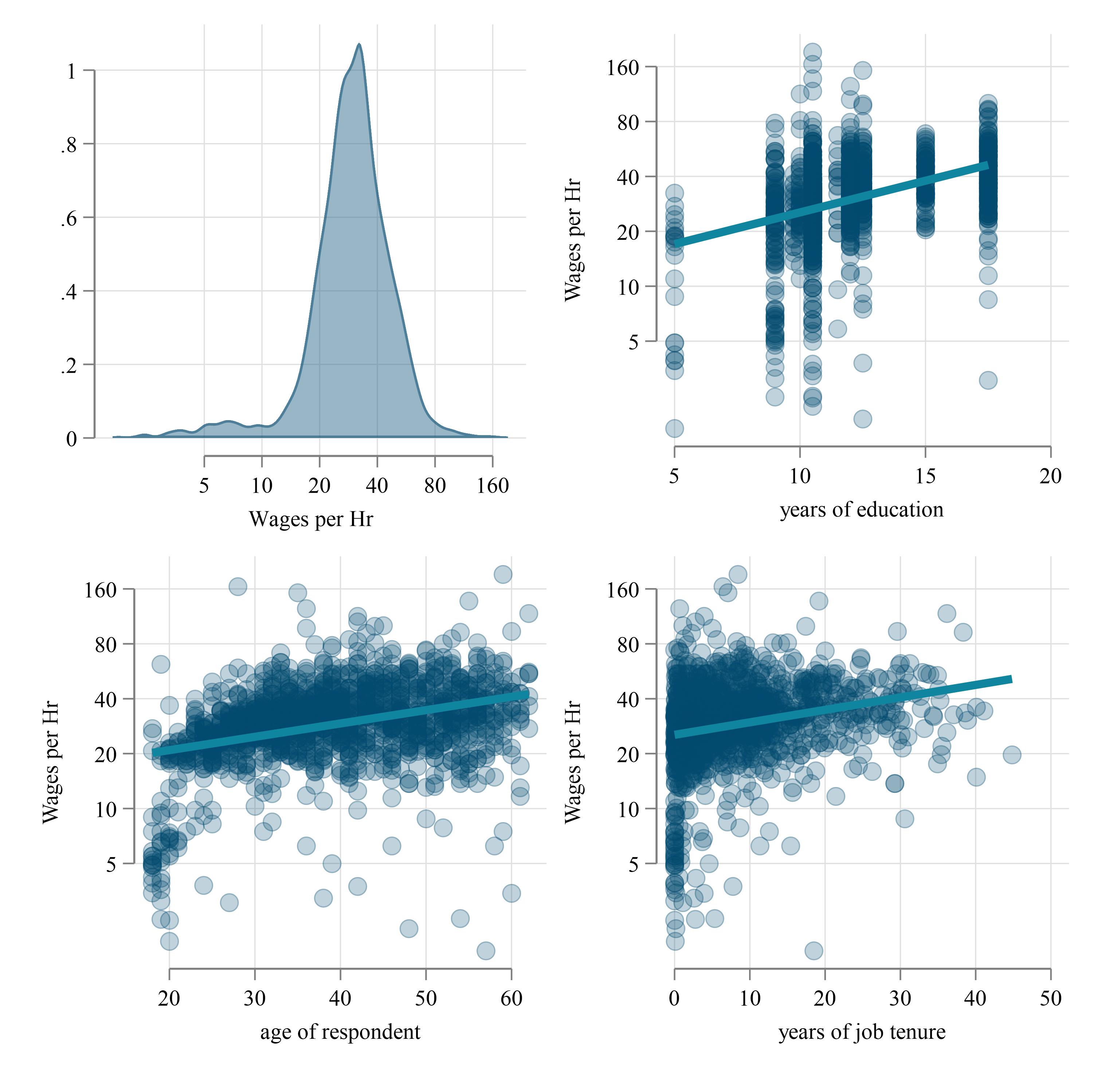

Figure 1 presents information on the visual correlations between wages and three of the varialbes of interest. Figure 1 (a) provides scatter plots of the fully observed wages agains the explanatory variables, whereas Figure 1 (b) does the same, but using the bracket censored data.
If one is interested in analyzing other moments, such as conditional quantiles, current methods would not allow for it, since they are mostly focused on explaining conditional means. However, that is where our approach comes into place. We start by using the intreg, het() command to model both the conditional mean and conditional variance. The latter is important because it allows us to explicitly model relationships between the dependent and independent variables that vary across the distribution. After we estimate the parameters for the conditional distribution, we can use it to generate multiple syntethic datasets (multiple imputation) with our command intreg_mi. This multiple imputed data can later be analyzed using standard econometric tools.
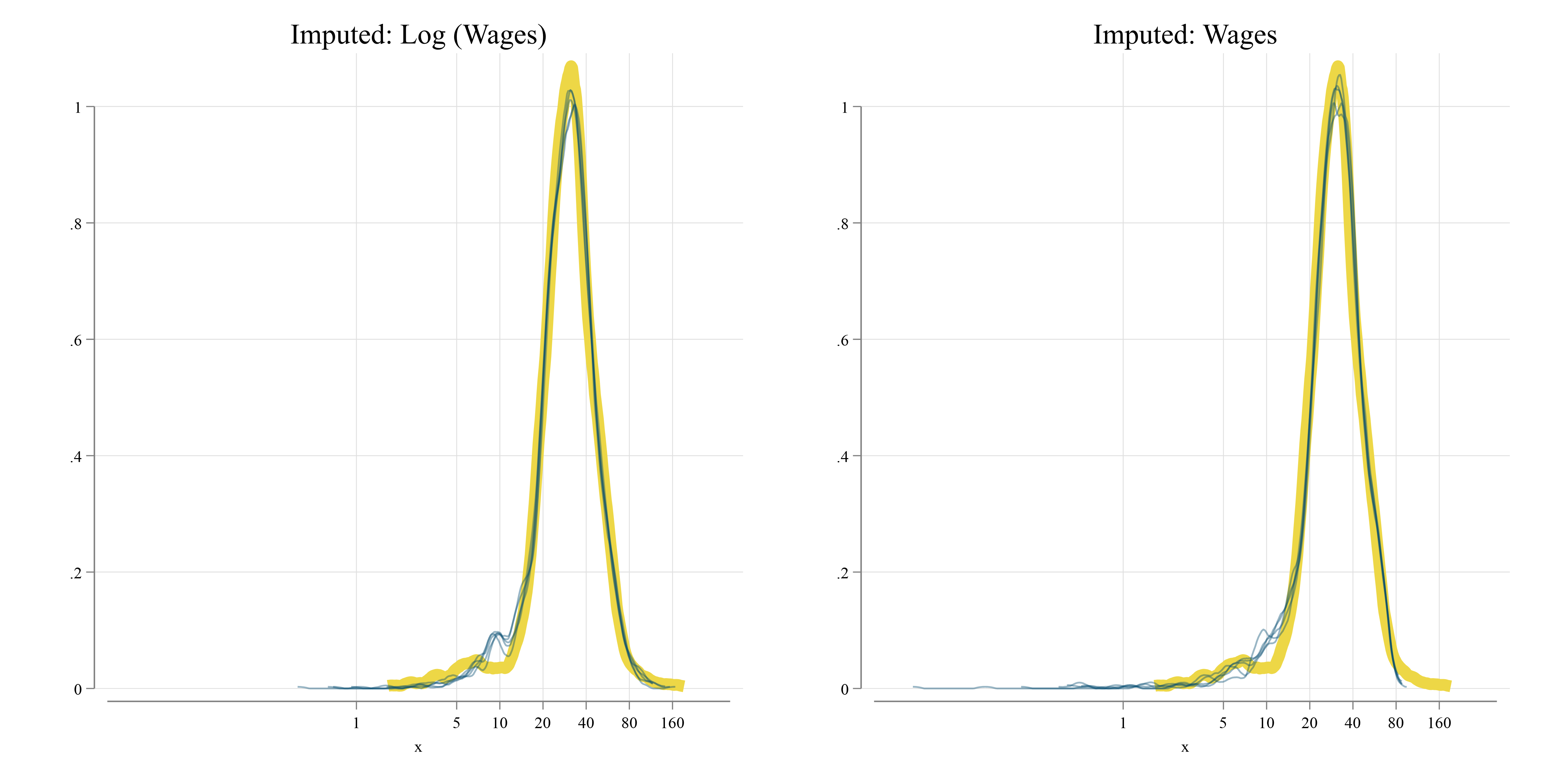
We use this strategy with the data from Figure 1 (b), and generate multiple synthetic datasets to reconstruct the censored data. For completeness, we impute directly wages as well as log(wages). To inspect how well the imputed data replicates the original data, we plot their density functions in Figure 2. The yellow line representing the true wage distribution, and the blue lines corresponding to the imputed data. And of this scenario, it seems that imputed log(wages), or wages directly has little effect in the replicating the wage distribution.
After creating the multiple-imputed synthethic datasets, they can be analyzed applying standard aggregation rules. In Stata, this can be done using mi commands. Because multiple imputation would provide no added value to the estimation of conditional means (linear regression), we compare esitmates using conditional quantile regressions.
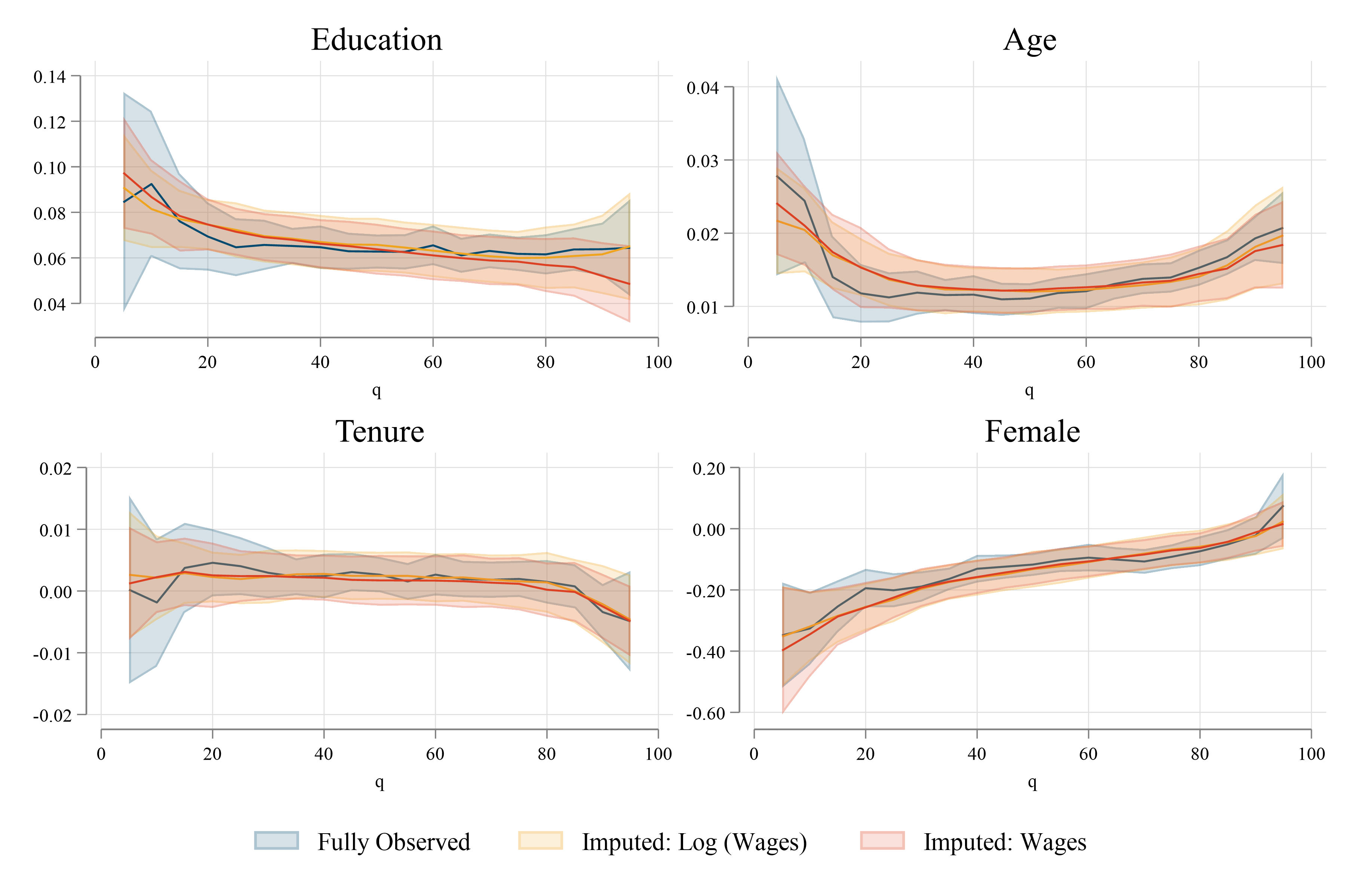
Figure 3 contrasts the results of the quantile regression coefficients, using the fully observed data, as well as the two imputed data options. In general, while the estimated parameters using imputed data does not replicate the quantile regression coefficients perfectly, it captures most of the observed trends across the distribution. Considering that we start with only limited information of wages in brackets, the fact that we can obtain good approximations of the unobserved effects is a considerable advantage.
The imputed data can be utilized in other ways. Policy analysists may be interested in analyzing the role of covariates on distributional statistics other than the mean. For example, they may be interested in analyzing income distribution using unconditional quantiles, Gini coefficients across groups, as well as other measures of income inequality.
| Fully Observed | Imp-log_w | Imp-wage | |
|---|---|---|---|
| Q_10 | 20.35 | 20.22 | 20.25 |
| (0.568) | (0.570) | (0.605) | |
| Q_90 | 52.72 | 52.51 | 52.37 |
| (1.126) | (1.561) | (1.295) | |
| Gini | 0.221 | 0.222 | 0.216 |
| (0.00677) | (0.00759) | (0.00672) | |
| Coeff of Variation | 0.413 | 0.422 | 0.392 |
| (0.0148) | (0.0197) | (0.0121) | |
| Log Variance | 0.238 | 0.221 | 0.268 |
| (0.0230) | (0.0242) | (0.0535) |
| Fully Observed | Imp-log_w | Imp-wage | |
|---|---|---|---|
| Q_10 | 15.87 | 13.98 | 13.57 |
| (0.576) | (0.850) | (0.815) | |
| Q_90 | 45.92 | 46.19 | 46.54 |
| (1.442) | (1.541) | (1.412) | |
| Gini | 0.267 | 0.254 | 0.249 |
| (0.0117) | (0.00950) | (0.00773) | |
| Coeff of Variation | 0.587 | 0.493 | 0.453 |
| (0.0461) | (0.0603) | (0.0141) | |
| Log Variance | 0.345 | 0.301 | 0.363 |
| (0.0347) | (0.0506) | (0.0637) |
Note: Standard Errors in Parenthesis
With this excercise in mind, Table 1 presents a few distributional statistics using the obseved and imputed data for men (Table 1 (a)) and women (Table 1 (b)). In all cases we obtain good approximations to the true statistics using the imputed data.
Conclusions
In our paper, we propose a method that makes better use of interval-censored. We propose using multiple imputation based on an interval-regression estimator with heteroskedastic errors, extending the work Royston (2007). The multiple imputed data can be used to analyze the heterogeneity across individual characteristics using regression tools such as conditional or unconditional quantile regressions.
In this note, we provide a small excercise of the type of analysis one could do using our approach. In the paper, we include further simulation evidence on the performance of the methodology, as well as real case study using data for the developing country of Grenada.
We believe that our method has important applications in economics and other social sciences, where interval-censored data are commonly used to capture income variables. Our method can also be used to analyze other types of censored data, such as duration data or survival data. We hope that our method will encourage more researchers to utilize interval-censored data in their research, and to develop more flexible and robust methods for analyzing such data.
Further Examples
As part of the journey of developing our method, we have produced a few examples that illustrate the application. You can find them in here:
Software
The excercise presented here was produce using Stata. The modeling was done using the official commands intreg. The imputed values were generated our command intreg_mi. The analysis of the data was performed using mi, qreg and rifhdreg.